DistClassiPy Tutorial

Author: Sid Chaini, October 22, 2024

This notebook gives a quick demo of using DistClassiPy to classify light curve features. For this demo, I will use the data from the Zwicky Transient Facility Source Classification Project (SCoPe, Healy et al. 2024).

0. Prerequisites

Let us first install DistClassiPy from PYPI. I am installing 0.2.1, the latest as of 2024-10-22

!pip install distclassipy==0.2.1 # latest as of 2024-10-22

Requirement already satisfied: distclassipy==0.2.1 in /Users/sidchaini/miniconda3/lib/python3.12/site-packages (0.2.1)
Requirement already satisfied: joblib>=1.3.2 in /Users/sidchaini/miniconda3/lib/python3.12/site-packages (from distclassipy==0.2.1) (1.4.2)
Requirement already satisfied: numpy>=1.25.2 in /Users/sidchaini/miniconda3/lib/python3.12/site-packages (from distclassipy==0.2.1) (1.26.4)
Requirement already satisfied: pandas>=2.0.3 in /Users/sidchaini/miniconda3/lib/python3.12/site-packages (from distclassipy==0.2.1) (2.2.2)
Requirement already satisfied: scikit-learn>=1.2.2 in /Users/sidchaini/miniconda3/lib/python3.12/site-packages (from distclassipy==0.2.1) (1.5.1)
Requirement already satisfied: python-dateutil>=2.8.2 in /Users/sidchaini/miniconda3/lib/python3.12/site-packages (from pandas>=2.0.3->distclassipy==0.2.1) (2.9.0.post0)
Requirement already satisfied: pytz>=2020.1 in /Users/sidchaini/miniconda3/lib/python3.12/site-packages (from pandas>=2.0.3->distclassipy==0.2.1) (2024.1)
Requirement already satisfied: tzdata>=2022.7 in /Users/sidchaini/miniconda3/lib/python3.12/site-packages (from pandas>=2.0.3->distclassipy==0.2.1) (2024.1)
Requirement already satisfied: scipy>=1.6.0 in /Users/sidchaini/miniconda3/lib/python3.12/site-packages (from scikit-learn>=1.2.2->distclassipy==0.2.1) (1.14.1)
Requirement already satisfied: threadpoolctl>=3.1.0 in /Users/sidchaini/miniconda3/lib/python3.12/site-packages (from scikit-learn>=1.2.2->distclassipy==0.2.1) (3.5.0)
Requirement already satisfied: six>=1.5 in /Users/sidchaini/miniconda3/lib/python3.12/site-packages (from python-dateutil>=2.8.2->pandas>=2.0.3->distclassipy==0.2.1) (1.16.0)

Let’s download a dataset I prepared from the ZTF SCoPE data for this tutorial.

%%capture
!wget https://github.com/sidchaini/DistClassiPyTutorial/archive/refs/heads/main.zip
!unzip main.zip
!mv DistClassiPyTutorial-main/* .
!rm -rf main.zip DistClassiPyTutorial-main

import numpy as np

seed = 0
np.random.seed(seed)
import pandas as pd
import distclassipy as dcpy
import utils
import matplotlib.pyplot as plt
import seaborn as sns
from sklearn.model_selection import train_test_split
from sklearn.metrics import accuracy_score, f1_score

1. Visualizing 2D distance metric spaces

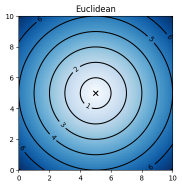
We can visualize the distance metric space by plotting the locus of a central point, such as (5, 5) in a given two dimensional space. The locus appear as contour lines, which can illustrate geometry of the space when plotted in Euclidean space.

utils.visualize_distance("euclidean")
plt.show()

2. Data

For this example, we will be using data from “The ZTF Source Classification Project: III. A Catalog of Variable Sources” through which they have made available on Zenodo.

I downloaded and sampled them to choose 4000 objects from 4 classes of variable stars:

features = pd.read_csv("data/ztfscope_features.csv", index_col=0)
labels = pd.read_csv("data/ztfscope_labels.csv", index_col=0)

labels.value_counts()

class
CEP      1000
DSCT     1000
RR       1000
RRc      1000
Name: count, dtype: int64

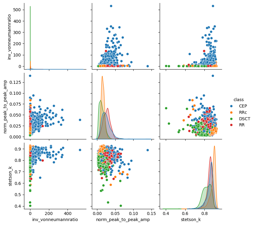
For the sake of simplicity, let us focus on three features from the complete ZTF SCoPE features (refer to Healy et al. 2024 for more details): - inv_vonneumannratio: Inverse of von Neumann ratio (von Neumann 1941, 1942), which is the ratio of correlated variance and variance - it detects non-randomness, and a high value implies periodic behaviour. - norm_peak_to_peak_amp: Normalized peak-to-peak amplitude (Sokolovsky et al. 2009) - it tells us about the source brightness. - stetson_k: Stetson K coefficient (Stetson 1996) is related to the observed scatter - it tells us about the light curve shape.

feature_names = ["inv_vonneumannratio", "norm_peak_to_peak_amp", "stetson_k"]

df = features.loc[:, feature_names]
df["class"] = labels["class"]
sns.pairplot(df, hue="class")
plt.show()

X = features.loc[:, feature_names].to_numpy()
y = labels.to_numpy().ravel()

X_train, X_test, y_train, y_test = train_test_split(
    X, y, test_size=0.25, random_state=seed
)

3. DistanceMetricClassifier

The DistanceMetricClassifier calculates the distance between a centroid for each class, and each test point, and scales it by the standard deviation.

clf = dcpy.DistanceMetricClassifier()
clf.fit(X_train, y_train)

DistanceMetricClassifier()

In a Jupyter environment, please rerun this cell to show the HTML representation or trust the notebook.
On GitHub, the HTML representation is unable to render, please try loading this page with nbviewer.org.

y_pred = clf.predict_and_analyse(X_test, metric="euclidean")

acc = accuracy_score(y_true=y_test, y_pred=y_pred)
f1 = f1_score(y_true=y_test, y_pred=y_pred, average="macro")

print(f"Accuracy = {acc:.3f}")
print(f"F1 = {f1:.3f}")

Accuracy = 0.642
F1 = 0.635

clf.centroid_dist_df_

	CEP_dist	DSCT_dist	RR_dist	RRc_dist
0	0.805759	2.641208	0.824424	2.848626
1	1.220526	1.423540	2.151157	1.164521
2	1.325282	3.792195	1.503853	4.076885
3	1.064865	8.376741	1.781160	1.323827
4	0.480929	2.229321	0.915641	2.055988
...	...	...	...	...
995	1.015133	3.548696	1.743593	0.106400
996	0.957050	10.627296	1.705001	1.205451
997	0.810418	14.319456	1.574726	1.767178
998	1.023541	2.556731	1.699193	0.937611
999	1.452081	1.219772	2.336256	2.059953

1000 rows × 4 columns

4. EnsembleDistanceClassifier

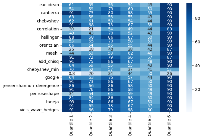
The EnsembleDistanceClassifier splits the training set into multiple quantiles based on a feature (feat_idx), iterates among all metrics to see which one performs the best on a validation set, and then prepares an ensemble based on the best performing metric for each quantile.

ensemble_clf = dcpy.EnsembleDistanceClassifier(feat_idx=0, random_state=seed)
ensemble_clf.fit(X_train, y_train, n_quantiles=6)

EnsembleDistanceClassifier(feat_idx=0, random_state=0)

In a Jupyter environment, please rerun this cell to show the HTML representation or trust the notebook.
On GitHub, the HTML representation is unable to render, please try loading this page with nbviewer.org.

y_pred_ensemble = ensemble_clf.predict(X_test)

acc = accuracy_score(y_true=y_test, y_pred=y_pred_ensemble)
f1 = f1_score(y_true=y_test, y_pred=y_pred_ensemble, average="macro")

print(f"Accuracy = {acc:.3f}")
print(f"F1 = {f1:.3f}")

Accuracy = 0.783
F1 = 0.783

ensemble_clf.best_metrics_per_quantile_

Quantile 1               taneja
Quantile 2         kumarjohnson
Quantile 3            hellinger
Quantile 4             canberra
Quantile 5    vicis_wave_hedges
Quantile 6            euclidean
dtype: object

ensemble_clf.quantile_scores_df_.drop_duplicates()

	Quantile 1	Quantile 2	Quantile 3	Quantile 4	Quantile 5	Quantile 6
euclidean	60.8	59.2	56.0	53.6	43.2	90.4
braycurtis	53.6	59.2	72.8	60.0	50.4	90.4
canberra	91.2	72.8	80.0	68.0	59.2	90.4
cityblock	63.2	58.4	56.0	55.2	43.2	90.4
chebyshev	62.4	60.8	57.6	53.6	44.0	90.4
clark	91.2	68.0	77.6	67.2	57.6	90.4
correlation	30.4	20.8	53.6	48.8	44.0	83.2
cosine	48.8	43.2	69.6	52.0	43.2	90.4
hellinger	88.0	68.0	85.6	67.2	49.6	90.4
jaccard	52.8	64.8	70.4	58.4	49.6	90.4
lorentzian	65.6	54.4	56.0	55.2	44.0	90.4
marylandbridge	24.8	18.4	40.0	37.6	41.6	87.2
meehl	44.0	52.8	57.6	62.4	46.4	90.4
wave_hedges	91.2	72.0	79.2	65.6	56.8	87.2
add_chisq	91.2	75.2	85.6	67.2	48.0	90.4
acc	64.0	59.2	55.2	55.2	43.2	90.4
chebyshev_min	70.4	52.0	56.8	36.8	40.8	52.8
dice	0.8	20.0	34.4	44.0	50.4	26.4
google	64.0	63.2	75.2	56.8	44.0	89.6
jeffreys	91.2	72.8	85.6	67.2	49.6	90.4
jensenshannon_divergence	85.6	66.4	85.6	68.0	50.4	90.4
kumarjohnson	91.2	76.0	85.6	68.0	48.8	90.4
penroseshape	34.4	53.6	60.8	59.2	48.8	90.4
prob_chisq	80.8	64.0	85.6	68.0	50.4	90.4
taneja	92.8	74.4	85.6	67.2	50.4	90.4
vicis_symmetric_chisq	91.2	64.8	77.6	67.2	56.8	90.4
vicis_wave_hedges	91.2	66.4	79.2	68.0	60.0	90.4

sns.heatmap(
    ensemble_clf.quantile_scores_df_.drop_duplicates(), annot=True, cmap="Blues"
)
plt.show()